§ 01 · Hook
September 2008. The S&P 500 lost 30% in three weeks.
Most systematic strategies were fully invested when the crash hit. This system detected the regime shift six days earlier. By September 19, allocation had dropped from 85% to 12%.
Why this matters
A 50% drawdown requires a 100% gain to recover. Most quant strategies fail because they confuse calm volatility with structural stability. Regime detection decouples the two.
▼−29%
Market · Sep–Dec 2008
▼−4.3%
Strategy · Sep–Dec 2008
▼−55%
Buy & Hold Max DD
▼−28%
Strategy Max DD
§ 02 · Performance
Equity curves, after costs.
Benchmarks
5 strategies tested against SPY buy and hold over 15 years of out of sample data. All results include 7 bps transaction costs and 1 day execution lag.
Hover for daily values. Click the legend to toggle strategies. Drag to zoom.
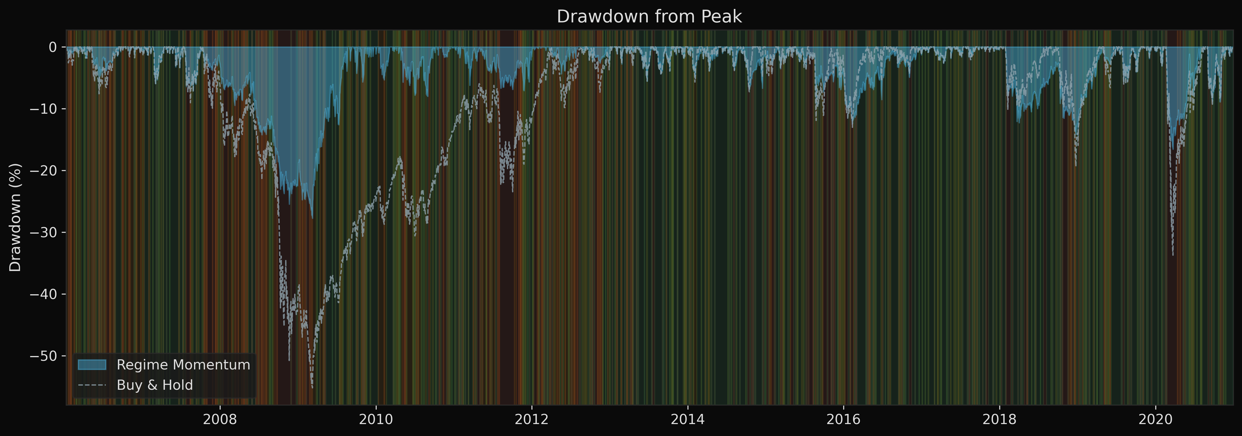
Drawdown from peak. Buy and hold hit −55% in 2008. The regime strategy cut that in half while delivering higher returns (10.2% vs 9.6% CAGR).
| Strategy | CAGR | Vol | Sharpe | Max DD | Turnover |
|---|---|---|---|---|---|
| Regime Momentum | 10.2% | 9.3% | 0.70 | −27.7% | 5.7× |
| Binary Regime | 7.5% | 12.5% | 0.49 | −35.8% | 10.6× |
| Vol-Managed | 6.6% | 10.5% | 0.47 | −23.7% | 1.7× |
| SMA 200 | 7.0% | 11.7% | 0.47 | −21.9% | 6.0× |
| Buy & Hold (SPY) | 9.6% | 20.1% | 0.45 | −55.2% | 0.0× |
§ 03 · Signal
Lead time
Median regime-shift detection occurs 6 trading days before peak drawdown. The asymmetric filter requires 3 consecutive turbulent signals to reduce exposure, but only 1 calm signal to re-enter.
Allocation leads drawdown.
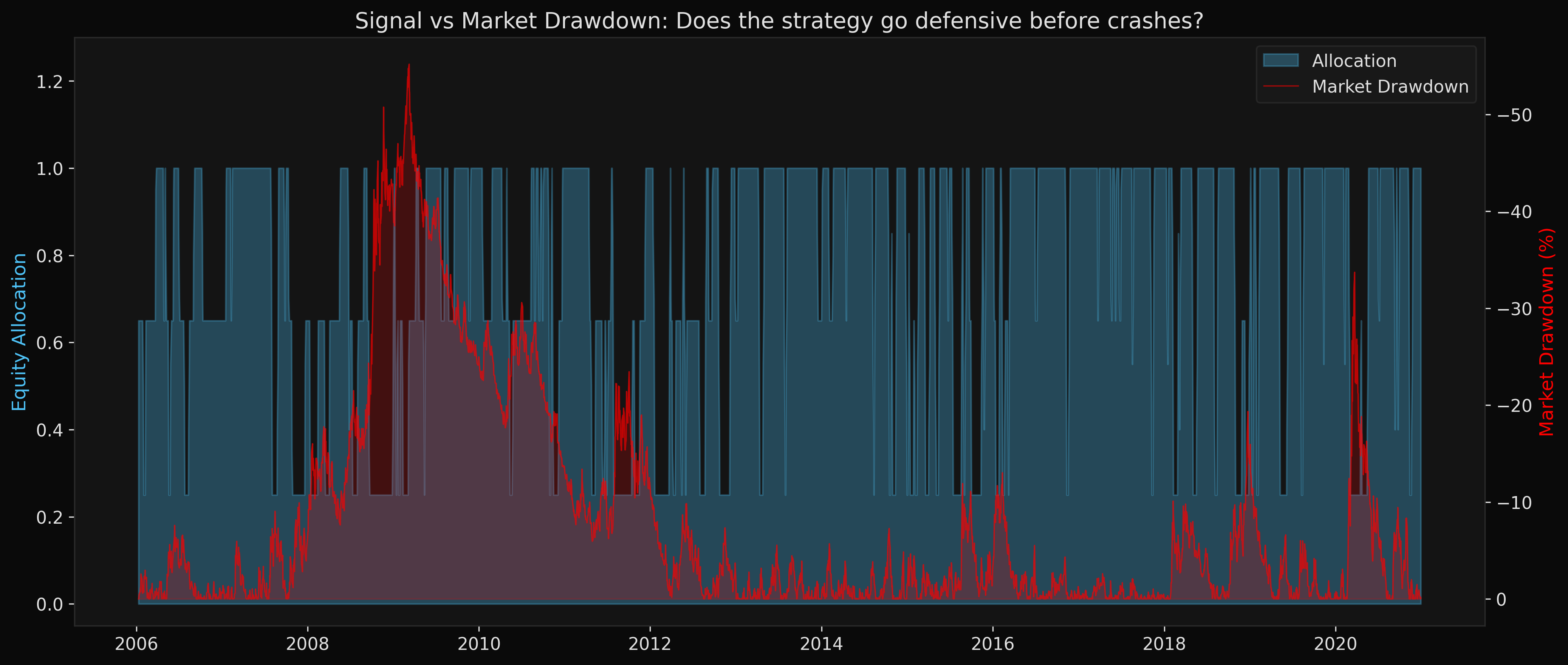
Bone: equity allocation. Terracotta: market drawdown. The strategy reduces exposure before and during every major drawdown of the sample.
§ 04 · Architecture
Five models, one ensemble.
190 Stocks
→
6 Features
→
5 Models
→
Ensemble
→
Signal
→
Backtest
- HMM · 5-state Gaussian, remapped to 3, transition persistence Feature-space
- GARCH(1,1) Student-t · conditional volatility clustering Return-based
- K-Means · feature-space clustering Feature-space
- Gaussian Mixture Model · Bayesian posterior probabilities Feature-space
- Markov-Switching · Hamilton 1989, regime-dependent variance Return-based
Walk forward validation, expanding window, quarterly refit. 59 windows, 3,771 out of sample predictions. SPY benchmark. 1 day execution lag. Asymmetric confirmation filters.
Walk forward loop
while train_end_idx + step_days <= n_total:
    train = feature_df.iloc[:train_end_idx]
    test  = feature_df.iloc[train_end_idx:test_end_idx]

    probs = {
        "hmm":    fit_predict_hmm(train, test),
        "garch":  fit_predict_garch(train, test),
        "kmeans": fit_predict_kmeans(train, test),
        "gmm":    fit_predict_gmm(train, test),
        "ms":     fit_predict_markov_switching(train, test),
    }
    combined = ensemble.combine(probs)
    train_end_idx += 63   # quarterly
§ 05 · Prediction
Regime forecast is real.
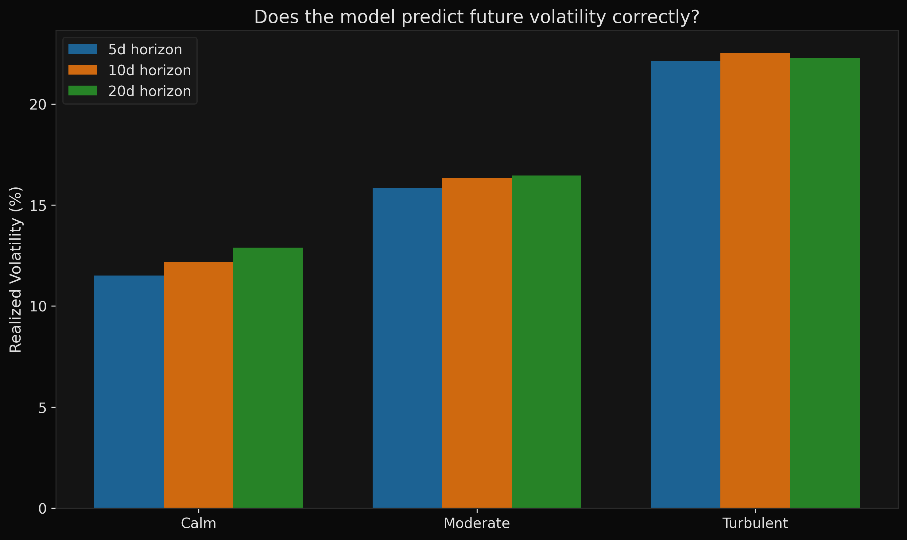
Realised volatility over the next 5, 10, and 20 days by predicted regime. Calm: 12%. Turbulent: 22%. Clear separation across all horizons.
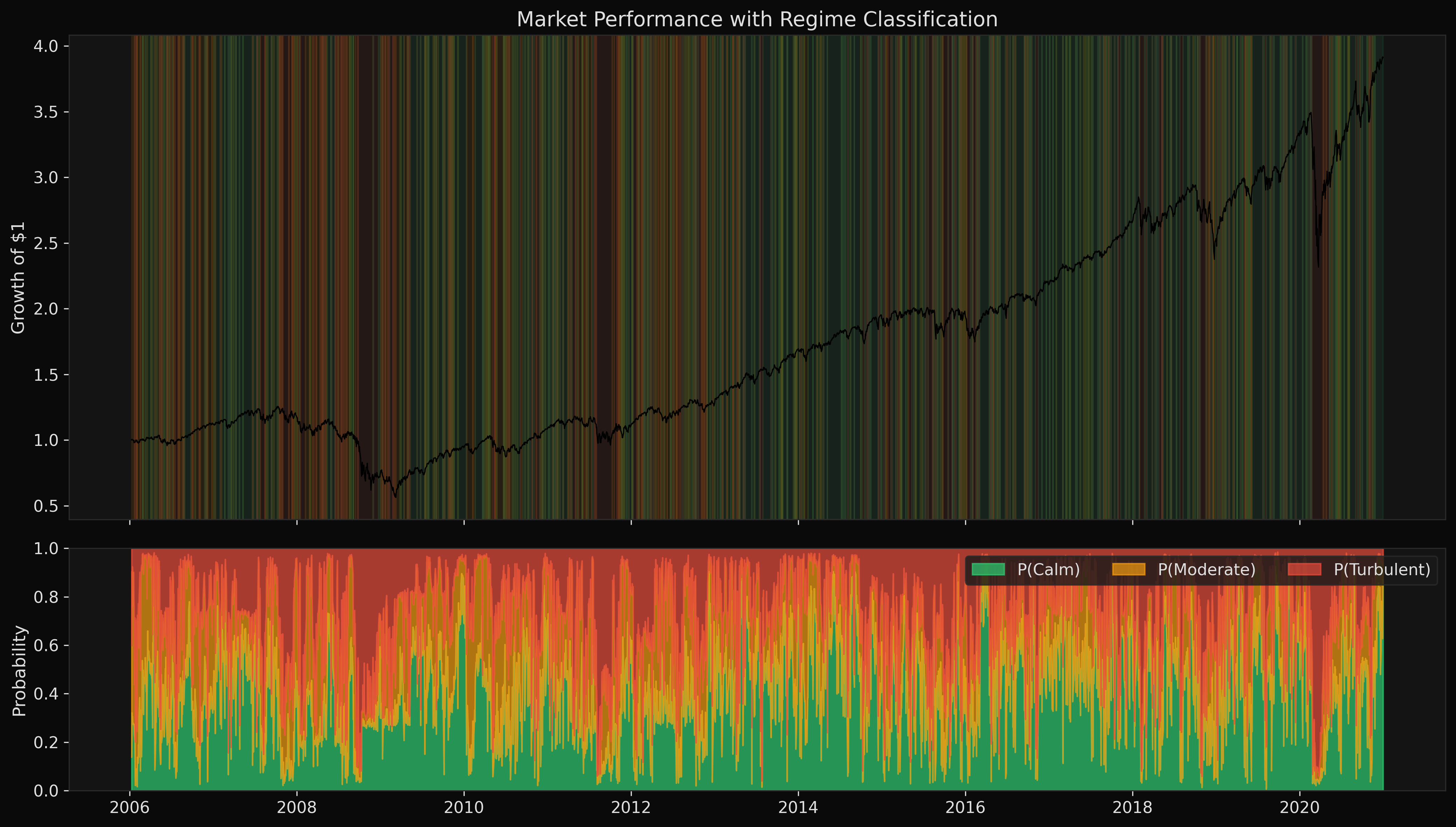
SPY with regime shading. Bottom panel: ensemble probability decomposition. Turbulent regimes concentrate around 2008, 2011, 2015, and early 2020.
§ 06 · Conditional Performance
Most returns come from calm regimes.
1.10
Calm Sharpe
52%
Trading Days Calm
81%
Return From Calm
0.18
Turbulent Sharpe
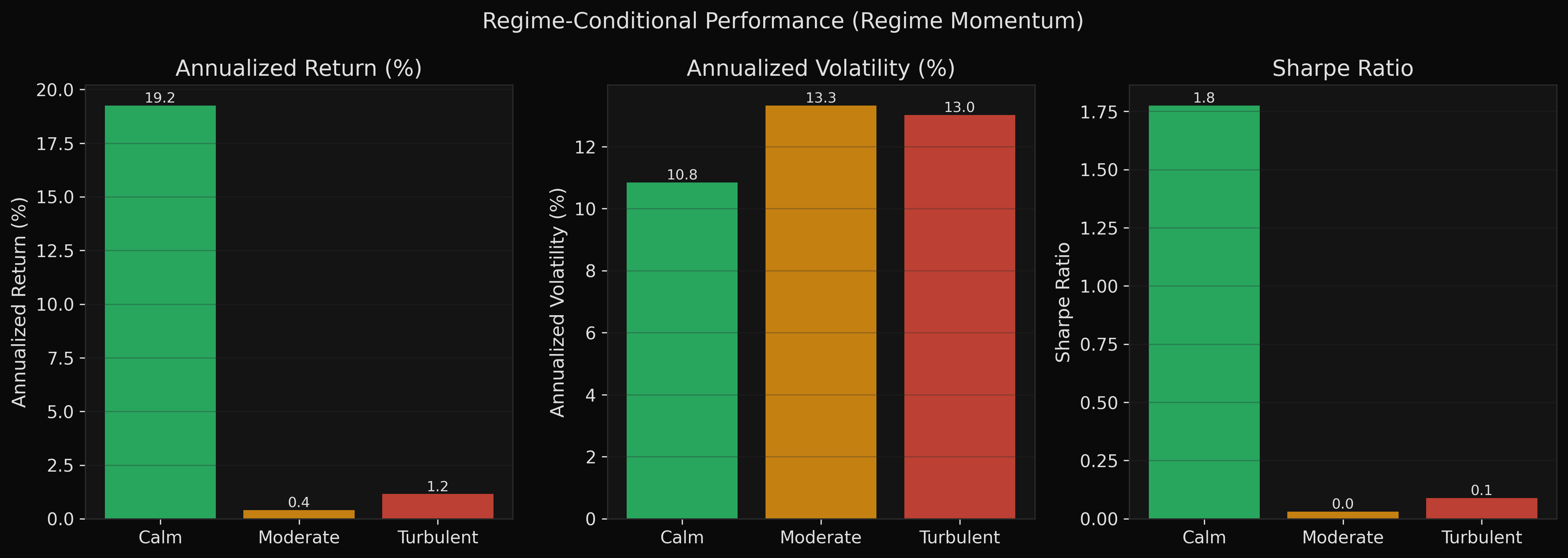
Calm markets: Sharpe 1.10. 81% of total return comes from 52% of trading days.
§ 07 · Cost Sensitivity
How much friction can it take?
Drag the slider to see how transaction costs affect performance. Institutional equity costs are typically 5 to 10 bps.
0.70
Sharpe
10.2%
CAGR
−28%
Max DD
31 bps
Breakeven
§ 08 · Stress Test
Through the 2008 crisis.
$10,000 invested in September 2007, right before the worst financial crisis in modern history.
$10,000
Regime Strategy
$10,000
SPY Buy & Hold
+46%
Alpha by 2010
2008-09
Worst 12 months
§ 09 · Cross-Asset
Same machinery, different market.
Demonstration extension
As a demonstration, I refit the same architecture on WTI crude oil without changing the model design. The goal was to test whether the regime framework could identify major commodity stress periods, not to make the commodity backtest the main result.
2008
Crash detected
2014–16
Oil glut flagged
2020
Negative price event
0.25
VIX correlation
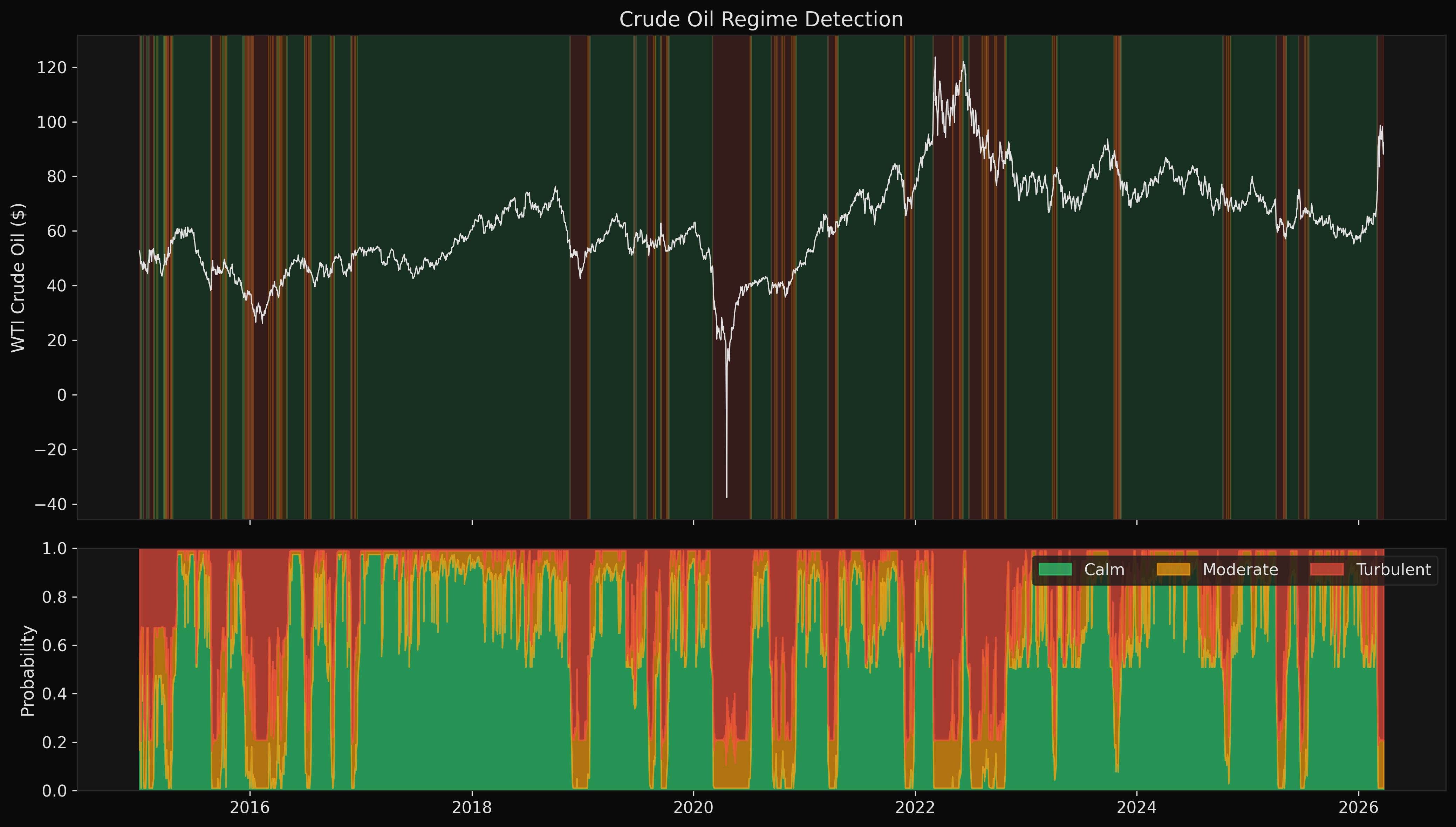
WTI crude oil regime detection. Correctly identifies the 2008 crash, the 2014–2016 oil glut, and the 2020 negative price event. Cross-asset correlation with equity VIX: 0.25.
§ 10 · Diagnostics
Ensemble agrees, then disagrees, then agrees.
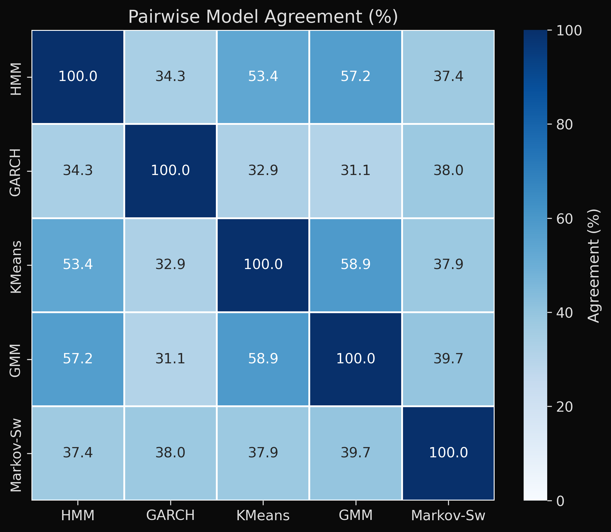
Pairwise agreement between the 5 models. Feature-space models (HMM, GMM) and return-based models (GARCH, Markov-Switching) form 2 independent clusters. Healthy diversification.
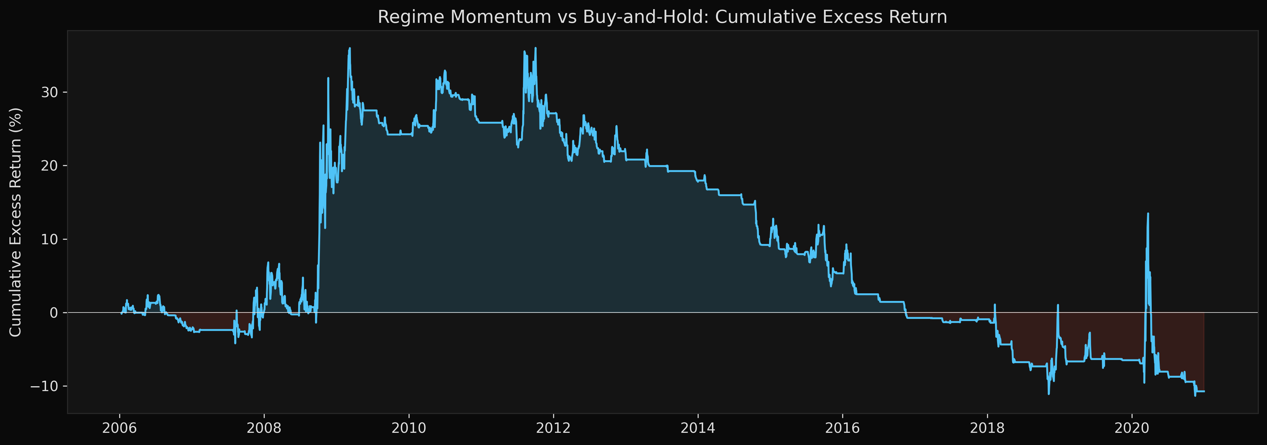
Cumulative excess return vs SPY. Alpha concentrates during crisis periods. Fama-French R-squared of 0.20 confirms low factor exposure.